Example for reading clm-file for example Tol

The clm.nc file is read and variable is extracted. Next, the mesh data is manipulated, converted to a raster and saved to a .tiff.

Manipulation of the mesh data includes obtaining the arrival time, the maximum rising speed, and the water height h_mrs at which this happen.

1. Import modules

import os
import sys
from pathlib import Path

import numpy as np

currentdir = os.path.dirname(os.getcwd())
sys.path.append(currentdir + r"/HydroLogic_Inundation_toolbox")
sys.path.append(currentdir + r"/HydroLogic_Inundation_toolbox/Readers")

from flowmeshreader import load_meta_data, load_classmap_data, mesh_to_tiff
from inundation_toolbox import arrival_times, height_of_mrs, rising_speeds
from plotting import raster_plot_with_context

2. Set input and output paths

# set paths
input_file_path = currentdir + r"/HydroLogic_Inundation_toolbox/Data/Tol/input/1PT10_clm.nc"
output_file_path = currentdir + r"/HydroLogic_Inundation_toolbox/Data/Tol/output"
Path(output_file_path).mkdir(exist_ok=True)

3. Set output raster options

# raster options
resolution = 10  # m
distance_tol = 36  # m
interpolation = r"nearest"

4. Read meta-data and set variable to read from clm.nc file

print(load_meta_data(input_file_path))
variable = r"Mesh2d_waterdepth"

['Mesh2d_flowelem_ba', 'Mesh2d_flowelem_bl', 'Mesh2d_s1', 'Mesh2d_waterdepth', 'Mesh2d_ucmag', 'Mesh2d_ucdir']

5. Load classmap and map data from NetCDF file

# load mesh coordinates and data from netCDF 
clm_data, map_data = load_classmap_data(input_file_path, variable, method="lower")

6. Compute arrival times, maximum rising speed, and waterheight at maximum rising speed

# Compute inundation specific variables
t_arrival = arrival_times(clm_data, np.timedelta64(60, "s"), time_unit="h", arrival_threshold=3)

s_rising = rising_speeds(map_data, time_step = np.timedelta64(60, "s"))
max_s_rising = np.amax(s_rising, axis=0)

h_mrs = height_of_mrs(map_data, s_rising)

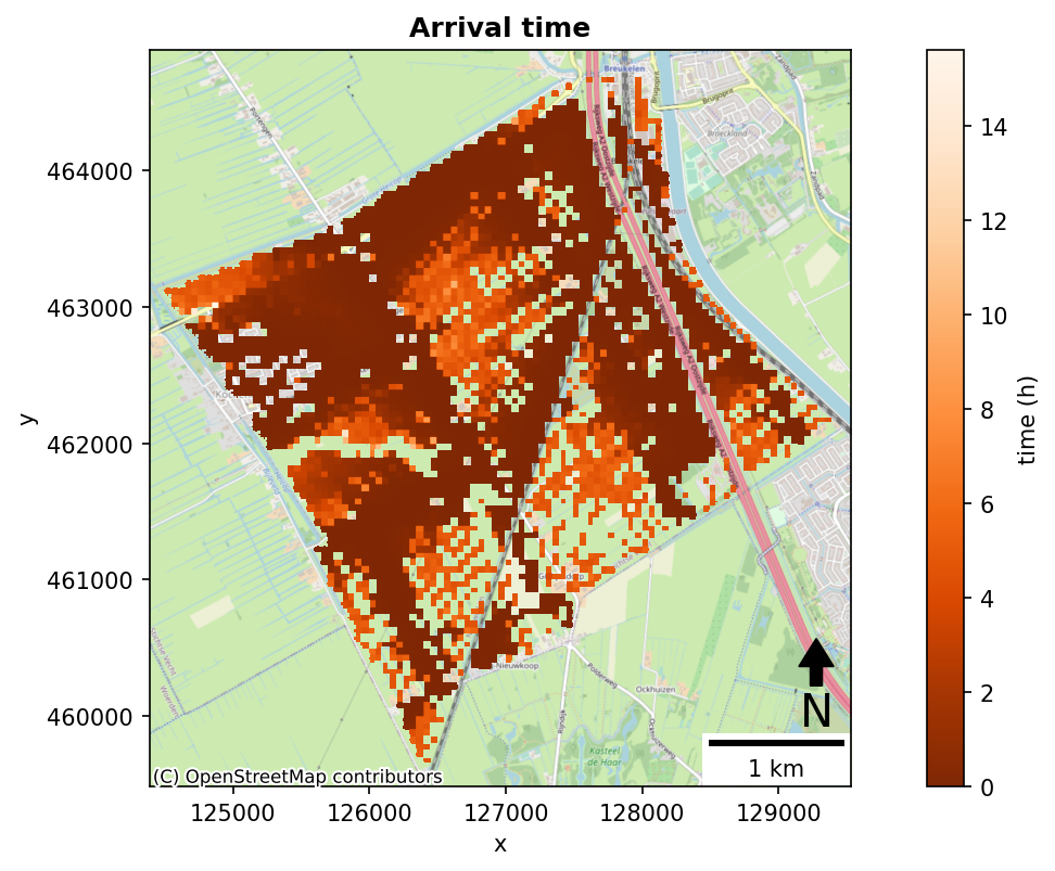
7. Plot Arrival time

# Plot arrival times
_, _, _ = mesh_to_tiff(
        t_arrival,
        input_file_path,
        output_file_path + r"/arrival.tiff",
        resolution,
        distance_tol,
        interpolation=interpolation,
    )
fig, ax = raster_plot_with_context(
    raster_path = output_file_path + r"/arrival.tiff", 
    epsg = 28992, 
    clabel = "time (h)", 
    cmap = "Oranges_r", 
    title = "Arrival time",
    )

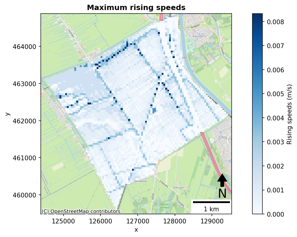
8. Plot Maximum rising speeds

# Plot maximum rising speeds
_, _, _ = mesh_to_tiff(
        max_s_rising,
        input_file_path,
        output_file_path + r"/max_rising.tiff",
        resolution,
        distance_tol,
        interpolation=interpolation,
    )
fig, ax = raster_plot_with_context(
    raster_path = output_file_path + r"/max_rising.tiff", 
    epsg = 28992, 
    clabel = "Rising speeds (m/s)", 
    cmap = "Blues", 
    title = "Maximum rising speeds",
    )

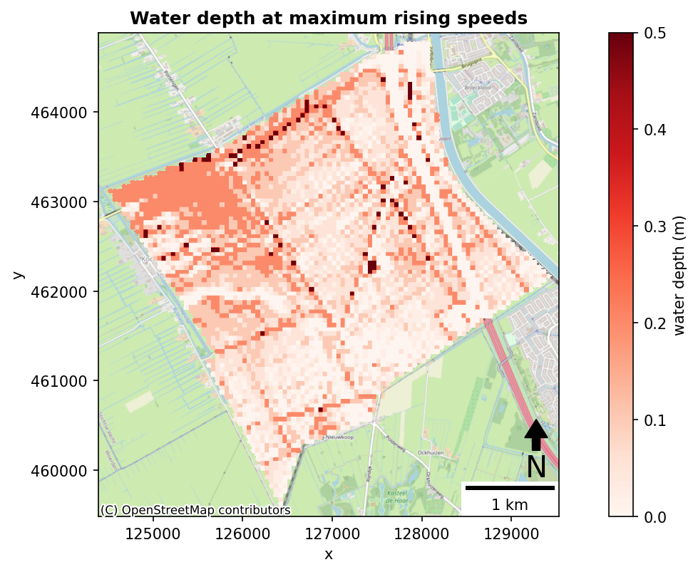
9. Plot water depth at maximum rising speeds

# Plot water depth of maximum rising speed
_, _, _ = mesh_to_tiff(
        h_mrs,
        input_file_path,
        output_file_path + r"/h_mrs.tiff",
        resolution,
        distance_tol,
        interpolation=interpolation,
    )
fig, ax = raster_plot_with_context(
    raster_path = output_file_path + r"/h_mrs.tiff", 
    epsg = 28992, 
    clabel = "water depth (m)", 
    cmap = "Reds", 
    title = "Water depth at maximum rising speeds",
    )